Predict spawning

Introduction

hatchR has a built in function—predict_spawn()—which allows users to predict when a fish’s parent spawned based on the observation of either when a fish hatched or emerged. The function works almost exactly the same as predict_phenology() but walks backwards from the point of development (hatch or emerge) and outputs spawn date.

Workflow

predict_spawn() works in essentially the same fashion as you learned about for predict_phenology() in the Predict fish phenology: basic vignette. First you have to select a developmental model. This will be determined by what life history stage from which you have empirical phenology data. For example, maybe you snorkeled a stream and observed bull trout emerging from a redd.

Model selection

Because our empirical data are from observing juvenile bull trout emergence we will use the bull trout emergence model using model_select() and our model_table. However, if you have custom models those could be used in the same fashion.

#select bull trout emergence model
bt_emerge_mod <- model_select(author = "Austin et al. 2019",
                                      species = "bull trout",
                                      model = "MM",
                                      development_type = "emerge"
                              )

We’ll use our crooked_river data set, which is temperature data from a reach of spawning bull trout. With model in hand we’ll predict spawn timing assuming we observed fish emerging March 21, 2015.

#predict spawn timing using "2015-03-21" emergence date
bt_spawn <- predict_spawn(data = crooked_river,
              dates = date,
              temperature = temp_c,
              develop.date = "2015-03-21",
              model = bt_emerge_mod
              )

The outputted object has the exact same structure as a predict_phenology() output. They include the slots:

days_to_develop: days from hatch or emergence to spawn
dev_period: a 1x2 dataframe where start= predicted spawn time and stop=empirical developmental event used for prediction in the model.
ef_table: a n x 5 tibble where n is the number of days from spawn to development. Note that the table is ordered from the development date and moves backwards in time. The columns are:
- index: the row number in the temperature data set
- dates: dates imported from your temperature data
- temperature: daily average temperature imported from your temperature data
- ef_vals: every day’s individual effective value
- ef_cumsum: the cumulative sum of effective values moving backwards from 1, a fish hatches when ef_cumsum <= 0.
model_specs: model specifications imported from the developmental model provided to predict_phenology()

A summary of the above output for bt_spawn is presented below.

str(bt_spawn)
#> List of 4
#>  $ days_to_develop: int 188
#>  $ dev_period     :'data.frame': 1 obs. of  2 variables:
#>   ..$ start: POSIXct[1:1], format: "2014-09-15"
#>   ..$ stop : POSIXct[1:1], format: "2015-03-21"
#>  $ ef_table       : tibble [188 × 5] (S3: tbl_df/tbl/data.frame)
#>   ..$ index      : num [1:188] 1572 1571 1570 1569 1568 ...
#>   ..$ dates      : POSIXct[1:188], format: "2015-03-21" "2015-03-20" ...
#>   ..$ temperature: num [1:188] 2.25 1.97 1.78 2 2.02 2.06 1.97 1.93 1.64 1.79 ...
#>   ..$ ef_vals    : num [1:188] 0.00496 0.00479 0.00467 0.00481 0.00482 ...
#>   ..$ ef_cumsum  : num [1:188] 0.995 0.99 0.986 0.981 0.976 ...
#>  $ model_specs    : spc_tbl_ [1 × 5] (S3: spec_tbl_df/tbl_df/tbl/data.frame)
#>   ..$ author          : chr "Austin et al. 2019"
#>   ..$ species         : chr "bull trout"
#>   ..$ model_id        : chr "MM"
#>   ..$ development_type: chr "emerge"
#>   ..$ expression      : chr "1/exp(5.590 - (x  * 0.126))"
#>   ..- attr(*, "spec")=List of 3
#>   .. ..$ cols   :List of 5
#>   .. .. ..$ author          : list()
#>   .. .. .. ..- attr(*, "class")= chr [1:2] "collector_character" "collector"
#>   .. .. ..$ species         : list()
#>   .. .. .. ..- attr(*, "class")= chr [1:2] "collector_character" "collector"
#>   .. .. ..$ model_id        : list()
#>   .. .. .. ..- attr(*, "class")= chr [1:2] "collector_character" "collector"
#>   .. .. ..$ development_type: list()
#>   .. .. .. ..- attr(*, "class")= chr [1:2] "collector_character" "collector"
#>   .. .. ..$ expression      : list()
#>   .. .. .. ..- attr(*, "class")= chr [1:2] "collector_character" "collector"
#>   .. ..$ default: list()
#>   .. .. ..- attr(*, "class")= chr [1:2] "collector_guess" "collector"
#>   .. ..$ delim  : chr ","
#>   .. ..- attr(*, "class")= chr "col_spec"
#>   ..- attr(*, "problems")=<externalptr>

So we see, the fish took 188 days to emerge with a predicted spawning date of September 15, 2014.

# development time
bt_spawn$days_to_develop
#> [1] 188

# spawning date
bt_spawn$dev_period$start
#> [1] "2014-09-15 UTC"

Finally, because the model output is in essentially the same format as that from predict_phenology() it can be plotted using plot_phenology() .

plot_phenology(bt_spawn)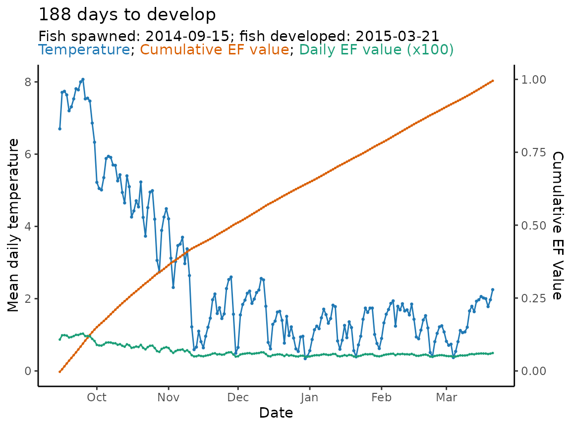

Compare to `predict_phenology()`

To demonstrate this provides the same information as predict_phenology() we can compare the outputs. Now we will use the predicted spawn date of "2014-09-15" as our input in predict_phenology().

bt_emerge <- predict_phenology(data = crooked_river,
              dates = date,
              temperature = temp_c,
              spawn.date = "2014-09-15",
              model = bt_emerge_mod
              )

And we can compare dev_period to verify the outputs match.

# are they the same (yes!)
bt_emerge$dev_period == bt_spawn$dev_period
#>      start stop
#> [1,]  TRUE TRUE

#print out values
bt_emerge$dev_period; bt_spawn$dev_period
#>        start       stop
#> 1 2014-09-15 2015-03-21
#>        start       stop
#> 1 2014-09-15 2015-03-21

Using multiple inputs for `predict_spawn()`

Like predict_phenology(), predict_spawn() can easily be mapped across multiple variable sets to automate the function. We can use a simple example of observing emerging fish across multiple months to demonstrate.

We’ll assume we observed fish emerging February 15, March 15, and April 15 in 2015. And then map() the function across those dates using the purrr package.

library(purrr)

#vector of dates
emerge_days <- c("2015-02-15","2015-03-15", "2015-04-15")

# object for predicting spawn timing across three emergence days
bt_multiple_emerge <- map(emerge_days, # vector of emergence dates
                          predict_spawn, # predict_spawn function
                          # everything below are arguments to predict_spawn()
                          data = crooked_river,
                          dates = date,
                          temperature = temp_c,
                          model = bt_emerge_mod)

# we can access just the dev_periods using map_df
# the start column provides the predicted spawn dates
bt_multiple_emerge |> 
  map_df("dev_period")
#>        start       stop
#> 1 2014-08-29 2015-02-15
#> 2 2014-09-11 2015-03-15
#> 3 2014-09-27 2015-04-15

Based on our predictions, the fish spawned for our respective observed emergence dates on August 29, September 11, and September 27 in 2014.

predict_spawn() can be automated to greater extents just like with predict_phenology(). We recommend reading the Predict fish phenology: advanced vignette to review ways to map across multiple variables.

Predict spawning

Morgan Sparks, Bryan M. Maitland

Introduction

Workflow

Model selection