Introduction

Overview

hatchR is an R package that allows users to predict hatch and emergence timing for wild fishes, as well as additional tools to aid in those analyses. hatchR is intended to bridge the analytic gap of taking statistical models developed in hatchery settings (e.g., Beacham and Murray 1990) and applying them to real world temperature data sets using the effective value framework developed by Sparks et al. (2019). hatchR is also available as an interactive web application at https://elifelts.shinyapps.io/hatchR_demo/.

hatchR is designed to be flexible to achieve many applications. However, by virtue of being built as a scripting application, hatchR is able to tackle very large datasets relatively quickly and efficiently. That is, hatchR can be used to predict hatch and emergence timing for many fish species across many locations and years. These type of upstream analyses are covered in additional vignettes in this package. In this introductory vignette, we:

describes input data requirements
provide recommendations for importing data
review basic data checks
preview the full hatchR workflow covered in other vignettes

The generalized workflow for hatchR, including the steps below and in subsequent other vignettes, is shown below.

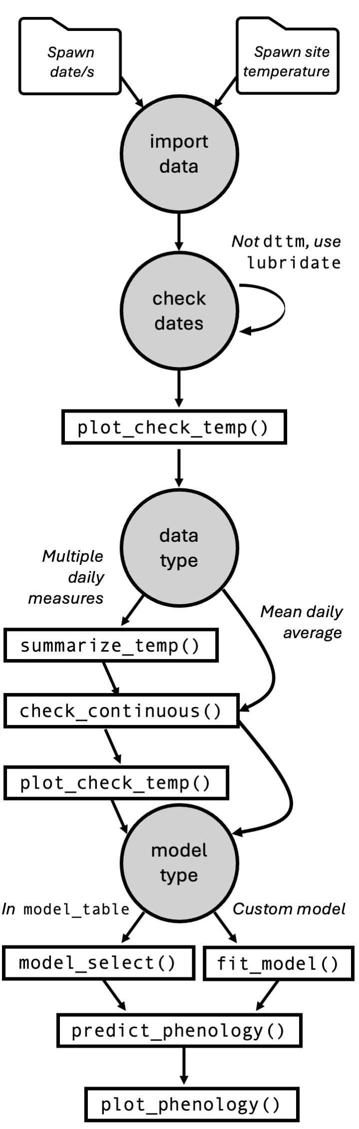
Input Data Requirements

hatchR requires three primary data inputs:

Water temperature data
Species-specific model parameters
Spawning date or date ranges

Water Temperature Data

Water temperature datasets for wild fishes are often either (1) already summarized by day (i.e., mean daily temperature) or, (2) in a raw format from something like a HOBO TidbiT data logger where readings are taken multiple times per day, which can be summarized into a mean daily temperatures. Alternatively, daily water temperature predictions from novel statistical models (e.g., Siegel et al. 2023) could be similarly implemented.

Fundamentally, hatchR assumes you have input data with two columns:

date: a vector of dates (and often times) of a temperature measurement (must be class Date or POSIXct, which Tibbles print as <date> and <dttm>, respectively).
temperature: a vector of associated temperature measurement (in centigrade).

Additional columns are allowed, but these are required.

We expect your data to look something like this:

date	temperature
2000-01-01	2.51
…	…
2000-07-01	16.32
…	…
2000-12-31	3.13

hatchR assumes you’ve checked for missing records or errors in your data because it can work with gaps, so it’s important to go through the data checks discussed below, as well as your own validity checks.

hatchR can use values down to freezing (e.g., 0 °C), which returns extremely small effective values, and time to hatch or emerge may be > 1 year. In these cases, we suggest users consider how much of that data type is reasonable with their data. To learn more about this, see the section on negative temperatures in the Predict fish phenology: Basic vignette.

Dates and Times

Numeric temperature values are simple to work with in R, but dates and time can be tricky. Here we provide a brief overview of how to work with dates and times in R, but refer the user to Chapter 17 in R for Data Science (Wickham, Çetinkaya-Rundel, and Grolemund 2023) for a more in-depth discussion.

The lubridate package makes it easier to work with dates and times in R. It comes installed with hatchR, and can be loaded with:

library(lubridate)

There are three types of date/time data that refer to an instant in time:

A date, which Tibbles print as <date>
A time within a day, which Tibbles print as <time>
A date-time is a date plus time, which Tibbles print as <dttm>. Base R calls these POSIXct, but that’s not a helpful name.

You can use lubridate::today() or lubridate::now() to get the current date or date-time:

today()
#> [1] "2025-02-27"
now()
#> [1] "2025-02-27 18:26:23 UTC"

In the context of hatchR, the ways you are likely to create a date/time are:

reading a file into R with readr::read_csv()
from a string (e.g., if data was read into R with read.csv())
from individual components (year, month, day, hour, minute, second)

Reading in dates from a file

When reading in a CSV file with readr::read_csv(), readr (which also comes installed with hatchR) will automatically parse (recognize) dates and date-times if they are in the form “YYYY-MM-DD” or “YYYY-MM-DD HH:MM:SS”. These are ISO8601 date (<date>) and date-time (<dttm>) formats, respectively. ISO8601 is an international standard for writing dates where the components of a date are organized from biggest to smallest separated by -. Below, we first load the readr package and then read in a CSV file with dates in the form “YYYY-MM-DD” and “YYYY-MM-DD HH:MM:SS”:

library(readr)

csv <- "
  date,datetime
  2022-01-02,2022-01-02 05:12
"
read_csv(csv)
#> # A tibble: 1 × 2
#>   date       datetime           
#>   <date>     <dttm>             
#> 1 2022-01-02 2022-01-02 05:12:00

If your dates are in a different format, you’ll need to use col_types plus col_date() or col_datetime() along with a standard date-time format (see Table 17.1 in R for Data Science (Wickham, Çetinkaya-Rundel, and Grolemund 2023) for a list of all date format options).

From strings

If you read in a CSV file using read.csv() from base R, date columns will be formatted as a characters (<char>; e.g., "2000-09-01" or "2000-09-01 12:00:00"). You will have convert to this column to a <date> or <dttm>. lubridate helper functions attempt to automatically determine the format once you specify the order of the component. To use them, identify the order in which year, month, and day appear in your dates, then arrange “y”, “m”, and “d” in the same order. That gives you the name of the lubridate function that will parse your date. For date-time, add an underscore and one or more of “h”, “m”, and “s” to the name of the parsing function.

ymd("2017-01-31")
#> [1] "2017-01-31"
mdy("January 31st, 2017")
#> [1] "2017-01-31"
mdy_hm("01/31/2017 08:01")
#> [1] "2017-01-31 08:01:00 UTC"
ymd_hms("2017-01-31 20:11:59")
#> [1] "2017-01-31 20:11:59 UTC"

From individual components

Sometimes you have the components of a date in separate columns. You can use make_date() or make_datetime() to combine them into a date or date-time.

To show this, we’ll use the flights dataset that comes with nycflights13, which is only installed alongside hatchR when dependencies = TRUE in install.packages(). We also make use of helper functions from dplyr to select() and mutate() columns.

library(nycflights13)
library(dplyr)

flights |> 
  select(year, month, day) |>
  mutate(date = make_date(year, month, day))
#> # A tibble: 336,776 × 4
#>    year month   day date      
#>   <int> <int> <int> <date>    
#> 1  2013     1     1 2013-01-01
#> 2  2013     1     1 2013-01-01
#> 3  2013     1     1 2013-01-01
#> 4  2013     1     1 2013-01-01
#> 5  2013     1     1 2013-01-01
#> # ℹ 336,771 more rows

flights |> 
  select(year, month, day, hour, minute) |> 
  mutate(departure = make_datetime(year, month, day, hour, minute))
#> # A tibble: 336,776 × 6
#>    year month   day  hour minute departure          
#>   <int> <int> <int> <dbl>  <dbl> <dttm>             
#> 1  2013     1     1     5     15 2013-01-01 05:15:00
#> 2  2013     1     1     5     29 2013-01-01 05:29:00
#> 3  2013     1     1     5     40 2013-01-01 05:40:00
#> 4  2013     1     1     5     45 2013-01-01 05:45:00
#> 5  2013     1     1     6      0 2013-01-01 06:00:00
#> # ℹ 336,771 more rows

Time Zones

Time zones are a complex topic, but we don’t need to delve too deep for our purposes. We will cover a few basic topics. For more information, see Chapter 17 in R for Data Science (Wickham, Çetinkaya-Rundel, and Grolemund 2023).

R uses the international standard IANA time zones. These use a consistent naming scheme {area}/{location}, typically in the form {continent}/{city} or {ocean}/{city}. Examples include “America/New_York”, “Europe/Paris”, and “Pacific/Auckland”.

You can find out what R thinks your current time zone is with Sys.timezone():

Sys.timezone()
#> [1] "UTC"

(If R doesn’t know, you’ll get an NA.)

In R, the time zone is an attribute of the date-time that only controls printing. For example, these three objects represent the same instant in time:

x1 <- ymd_hms("2024-06-01 12:00:00", tz = "America/New_York")
x1
#> [1] "2024-06-01 12:00:00 EDT"

Unless otherwise specified, lubridate always uses UTC. UTC (Coordinated Universal Time) is the standard time zone used by the scientific community and is roughly equivalent to GMT (Greenwich Mean Time). It does not have DST, which makes a convenient representation for computation. Thus read_csv() converts to UTC, so if times are shifted, then daily summaries can be incorrect. This only matters if data are not daily yet, as.posixct() sets to local time.

You can change the time zone in two ways:

Change the time zone attribute with force_tz()
Change the time zone for printing with with_tz()

Importing water temperature data

Using `readr::read_csv()`

We recommend loading your data into R using readr::read_csv(). We can load readr using:

library(readr)

In this and other vignettes, we will use two datasets that come installed with the package: crooked_river and woody_island. Each dataset is available to the user as R objects once hatchR is installed and attached (see ?crooked_river or ?woody_island for more information). The raw example data (.csv files) are stored in the extdata/ directory installed alongside hatchR. We may store the file paths to example data:

path_cr <- system.file("extdata/crooked_river.csv", package = "hatchR")
path_wi <- system.file("extdata/woody_island.csv", package = "hatchR")

After specifying path_* (using system.file()), we load the example dataset into R:

crooked_river <- read_csv(path_cr)
woody_island <- read_csv(path_wi)

We check the crooked_river dataset by running either str() or tibble::glimpse() to see the structure of the data. glimpse() is a little like str() applied to a data frame, but it tries to show you as much data as possible. We prefer tibble::glimpse() because it is more compact and easier to read. tibble also comes installed with hatchR.

library(tibble)

Now we can check the structure of the crooked_river dataset:

glimpse(crooked_river)
#> Rows: 1,826
#> Columns: 2
#> $ date   <dttm> 2010-12-01, 2010-12-02, 2010-12-03, 2010-12-04, 2010-12-05, 20…
#> $ temp_c <dbl> 1.1638020, 1.3442852, 1.2533443, 1.0068728, 1.2899153, 1.229158…
glimpse(woody_island)
#> Rows: 735
#> Columns: 2
#> $ date   <chr> "8/11/1990", "8/12/1990", "8/13/1990", "8/14/1990", "8/15/1990"…
#> $ temp_c <dbl> 25.850000, 23.308333, 18.533333, 15.350000, 13.966667, 11.35833…

For your own data, assuming you have a .csv file in a data folder in your working directory called your_data.csv, you would call:

library(readr)
library(tibble)
your_data <- read_csv("data/your_data.csv")
glimpse(your_data)

Using `read.csv()`

If you import your data in with functions like read.csv() or read.table(), date columns will be formatted as a characters (<chr>). You will have convert to this column to a <date> or <dttm> type, and we recommend you do this using lubridate, which makes dealing with date a litter easier.

Below is an example of how you might do this. First, we check the structure of the crooked_river and woody_island datasets:

crooked_river <- read.csv(path_cr)
woody_island <- read.csv(path_wi)

glimpse(crooked_river) # note date column imported as a character (<chr>)
#> Rows: 1,826
#> Columns: 2
#> $ date   <chr> "2010-12-01T00:00:00Z", "2010-12-02T00:00:00Z", "2010-12-03T00:…
#> $ temp_c <dbl> 1.1638020, 1.3442852, 1.2533443, 1.0068728, 1.2899153, 1.229158…
glimpse(woody_island) # note date column imported as a character (<chr>)
#> Rows: 735
#> Columns: 2
#> $ date   <chr> "8/11/1990", "8/12/1990", "8/13/1990", "8/14/1990", "8/15/1990"…
#> $ temp_c <dbl> 25.850000, 23.308333, 18.533333, 15.350000, 13.966667, 11.35833…

Then, we convert the date columns using lubridate:

# if your date is in the form "2000-09-01 12:00:00"
crooked_river$date <- ymd_hms(crooked_river$date)

# if your date is in the form "2000-09-01"
woody_island$date <- mdy(woody_island$date) 

glimpse(crooked_river)
#> Rows: 1,826
#> Columns: 2
#> $ date   <dttm> 2010-12-01, 2010-12-02, 2010-12-03, 2010-12-04, 2010-12-05, 20…
#> $ temp_c <dbl> 1.1638020, 1.3442852, 1.2533443, 1.0068728, 1.2899153, 1.229158…
glimpse(woody_island)
#> Rows: 735
#> Columns: 2
#> $ date   <date> 1990-08-11, 1990-08-12, 1990-08-13, 1990-08-14, 1990-08-15, 19…
#> $ temp_c <dbl> 25.850000, 23.308333, 18.533333, 15.350000, 13.966667, 11.35833…

Temperature data checks

After data are loaded and dates are formatted correctly, we can complete a series of checks to ensure that the temperature data is in the correct format and that there are no missing values.

hatchR provides several helper functions to assist with this process.

library(hatchR)

Visualize your temperature data

hatchR comes with the function plot_check_temp() to visualize your imported data and verify nothing strange happened during your import process. The function outputs a ggplot2 object which can be subsequently modified by the user. The arguments temp_min = and temp_max = can be used to custom set thresholds for expected temperature ranges (defaults are set at 0 and 25 °C). Here is an example using the built-in dataset crooked_river:

plot_check_temp(data = crooked_river, 
                dates = date, 
                temperature = temp_c, 
                temp_min = 0, 
                temp_max = 12)

Summarize temperature data

If you imported raw data with multiple recordings per day, hatchR has a built in function to summarize those data to a daily average mean called summarize_temp(). The output of the function is a tibble with mean daily temperature and its corresponding.

Below, we simulate a dataset with 30-minute temperature recordings for a year and summarize the data to daily means.

# set seed for reproducibility
set.seed(123)

# create vector of date-times for a year at 30 minute intervals
dates <- seq(
  from = ymd_hms("2000-01-01 00:00:00"),
  to = ymd_hms("2000-12-31 23:59:59"), 
  by = "30 min"
  )

# simulate temperature data
fake_data <- tibble(
  date = dates,
  temp = rnorm(n = length(dates), mean = 10, sd = 3) |> abs()
)

# check it
glimpse(fake_data)
#> Rows: 17,568
#> Columns: 2
#> $ date <dttm> 2000-01-01 00:00:00, 2000-01-01 00:30:00, 2000-01-01 01:00:00, 2…
#> $ temp <dbl> 8.318573, 9.309468, 14.676125, 10.211525, 10.387863, 15.145195, 1…

Now we can summarize the data to daily means using summarize_temp():

fake_data_sum <- summarize_temp(data = fake_data,
                                temperature = temp,
                                dates = date)

nrow(fake_data) #17568 records
#> [1] 17568
nrow(fake_data_sum) #366 records; 2000 was a leap year :)
#> [1] 366

We again recommend, at a minimum, visually checking your data once it has been summarized.

# note we use fake_data_sum instead of fake_data
plot_check_temp(data = fake_data_sum, 
                dates = date, 
                temperature = daily_temp, 
                temp_min = 5,
                temp_max = 15)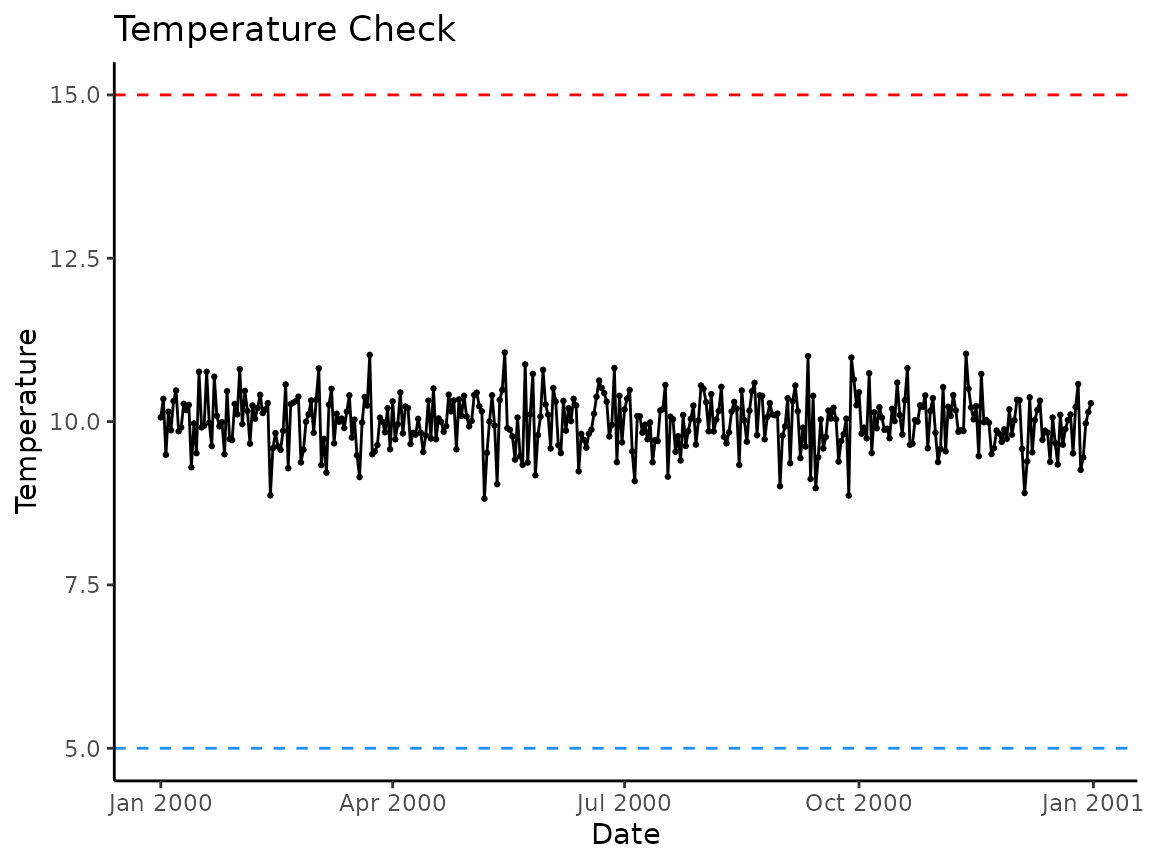

Check for continuous data

At present, hatchR only uses continuous data. Therefore, your data is expected to be continuous and complete.

You can check whether your data is complete and continuous using the check_continuous() function. This function will return a message if the data is or is not continuous or complete. Below, the calls return all clear:

check_continuous(data = crooked_river, dates = date)
#> ℹ No breaks were found. All clear!
check_continuous(data = woody_island, dates = date)
#> ℹ No breaks were found. All clear!

But if you had breaks in your data:

check_continuous(data = crooked_river[-5,], dates = date)
#> Warning: ! Data not continuous
#> ℹ Breaks found at rows:
#> ℹ 5

You’ll get a note providing the row index where breaks are found for inspection.

If you have days of missing data, you could impute them using rolling means or other approaches.

Species-specific model parameters

hatchR has two options for selecting parameterized models for predicting fish early life history phenology using:

model parameterizations included in the package
custom parameterizations using your own data

This processes is described in the vignette Parameterize hatchR models

Spawn Dates

A date or range of dates for spawning the species of interest is required to predict phenology. This information can be provided in the form of a single date or a range of dates. More information on how to provide this information is available in the vignette Predict phenology: basic, as well as subsequent vignettes.

Next steps

After importing, wrangling, and checking your temperature data, there are a number of different actions you can take. These steps are laid out in subsequent vignettes:

References

Beacham, Terry D., and Clyde B. Murray. 1990. “Temperature, Egg Size, and Development of Embryos and Alevins of Five Species of Pacific Salmon: A Comparative Analysis.” Transactions of the American Fisheries Society 119 (6): 927–45. https://doi.org/10.1577/1548-8659(1990)119<0927:TESADO>2.3.CO;2.

Siegel, Jared E., Aimee H. Fullerton, Alyssa M. FitzGerald, Damon Holzer, and Chris E. Jordan. 2023. “Daily Stream Temperature Predictions for Free-Flowing Streams in the Pacific Northwest, USA.” PLOS Water 2 (8): e0000119. https://doi.org/10.1371/journal.pwat.0000119.

Sparks, Morgan M., Jeffrey A. Falke, Thomas P. Quinn, Milo D. Adkison, Daniel E. Schindler, Krista Bartz, Dan Young, and Peter A. H. Westley. 2019. “Influences of Spawning Timing, Water Temperature, and Climatic Warming on Early Life History Phenology in Western Alaska Sockeye Salmon.” Canadian Journal of Fisheries and Aquatic Sciences 76 (1): 123–35. https://doi.org/10.1139/cjfas-2017-0468.

Wickham, Hadley, Mine Çetinkaya-Rundel, and Garrett Grolemund. 2023. R for Data Science. "O’Reilly Media, Inc.".

Morgan Sparks, Bryan M. Maitland